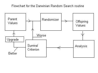
During the course of some work on a certain klystron, it became desirable to come up with a lumped element "equivalent" network to represent a distributed element 2-cavity network coupled to a waveguide. Walt Gasta and I presented a paper at the Monterey tube conference on our work toward this end. This presentation was brief and highly technical and not suitable for anyone not directly concerned with the issues. But I feel that the ideas and the results are, or should be, of much broader interest to some, thus this effort here.

Some technical discussion is, however, necessary (or so I feel) for my reader to grasp the full impact of my thesis. My introduction to "lumped element equivalent networks" came down from Jim Ebers, my professor and thesis advisor, when I was at Ohio State University in 1951. The specific course was entitled "Network Synthesis". I was pretty well versed in "Network Analysis" by this time. The problem in N.A. is this: given a network of specific elements and the driving function… the applied voltages and/or currents… find the response function. The problem in N.S. is this: given the driving function and the desired response, find the network elements. In the first case, the solution is almost always unique, while in the latter case the solution is generally impossible and usually an approximation at best. As graduate students, the class was abundantly familiar with lumped circuit elements, Inductors, L (Henries), Capacitors, C (Farads), and resistors, R (Ohms), as well as Voltages, V (Volts), and Currents, I (Amperes).

But any fundamental understanding of Electricity and Magnetism requires some understanding of Maxwell’s Equations. These are a set of partial differential equations in 4-dimensions (3-space and 1-time) describing Electric Fields, E (Volts/Meter), and Magnetic Fields, H (Ampere/Meter). A "Field" may be thought of as a region in space and time to which we may assign numerical values, magnitude and direction, to various quantities at each point. Many relatively simple solutions to Maxwell’s Equations, for certain geometries, are quite familiar to students of electrical engineering, but (except for electrolytic tank and deformable membrane analogs, etc.) the general solutions for more complex geometries were practically insoluble before the advent of fast digital computers and sophisticated software. Before this, Human Intuition was all-powerful.

Ebers once returned from his summer vacation and told several of his students of watching a school of porpoises leaping and playing ahead of the ship he was on somewhere in the South Pacific. How such marvelous creatures came to be was a great challenge to him, for one of his oft-repeated basic principles was that "things usually happen for a reason, unless, of course, they just happen". This latter proposition was, of course, pure anathema to us budding scientists.

Ebers built and studied a variety of vacuum tubes, called klystrons, in the Vacuum Tube Laboratory at Ohio State where I served as a graduate student-intern. The active element in his klystrons was an electron beam flowing through a resonant cavity coupled to an output waveguide. The electron beam excited an electric field in the cavity and some of the kinetic energy of the beam electrons was converted to electromagnetic energy that appeared as an electromagnetic wave in the output waveguide. This E-M wave was useful for all manner of stuff.

Almost any hardware configuration of like elements… electron beam, resonant cavity, and output waveguide… worked in some sense, but Ebers and all others at his level insisted on a theory to explain all or most of the observed performance. Without such a theory there was no meaningful understanding and no likelihood of fine tuning the performance of any specific device or branching off into new territory. The ideal procedure was a complete field solution coupled with the equations of motion and the applicable conservation laws of physics, but in those slide rule days and with time being recognized as money, almost no one could afford the luxury. Not everyone was wholly satisfied with this conclusion. Ebers’ and my boss, Prof. E. M. Boone, once reminded us of one of his heroes in science who compiled extensive tables of logarithms and trigonometric functions longhand over a period of years.

Ebers’ approach was to reduce the resonant cavity to a simple "equivalent" lumped element network and the electron beam and consequent Electric and Magnetic fields to Voltages and Currents. A resonant frequency and a loss factor, or "Q", could characterize the electro-magnetic fields in the cavity almost uniquely over a narrow, but more than adequate, band of frequencies. A simple lumped element network of an inductor, L, a capacitor, C, and a resistor, R, connected in parallel could be similarly characterized. If the stored energy in terms of the Electric and Magnetic fields in the cavity were made identical, the two devices were mathematically indistinguishable in the vicinity of the resonant frequency. The mathematics of network analysis was far simpler than field analysis while Voltages and Currents were far simpler to deal with than Electric and Magnetic fields and the equations of motion with regard to the electron beam. The subsequent theory of klystron behavior based on these ideas accurately predicted the behavior of the real devices and did, indeed, lead to the discovery of more and more advanced devices.

Another matter that interested Ebers greatly in his few idle hours was the protective coloration of certain creatures in nature. Boone liked to take his vacations climbing mountains out West or wandering over the cactus deserts in Arizona. He once brought in some photographs of horned toads barely visible against the background of the desert floor. Ebers later made the comment to a couple of his students that this probably happened for a reason, unless, of course, it just happened. He saw it as an advanced exercise in Network Synthesis thus: given the driving functions and the desired response, find the network elements. The driving function here was sunlight while the desired response was invisibility as referred to your predators, and the network elements were the myriad details of your coloration. He suggested that one-day, perhaps, we might have computers powerful and fast enough to address such problems in a meaningful way.

At the outset of the klystron project, a 2-cavity Extended Interaction Output Circuit, EIOC, had been built following our best understanding and intuition, but the actual response in terms of the output power across a specified band of frequencies fell short of the project requirements. It was not clear how to adjust the geometry to improve matters and the need for a lumped element model and an advanced analysis of beam kinetics to more precisely define the driving function was indicated. Our competitors, at Brand-X a few miles down the street, were following an approach based on a complete field analysis coupled with the electron beam kinetics. This analysis was based on the latest and most advanced PIC (Particle-In-Cell) software from the National Laboratories. A single case (frequency) could take up to 36 hours to converge. We did not have the luxury of the software or an operator who knew how to run it. In the end, this competitor told the customer that the goals of the project were impossible to meet.

Ebers was able to develop his klystron theory for a single cavity device based on a 3-element lumped equivalent model. When, in the 1990s, we tried to find a lumped element network to simulate a 2-cavity distributed network, the simplest network we could envision had at least 12 elements. Two of these elements, the interaction gaps, could be simulated reasonably well by capacitors that were found directly from a field analysis of the actual geometry, thanks to powerful fast computers and advanced software. This analysis was required only once, but we were left with 10 elements to find. From the Network Synthesis course I recalled, after some effort, that we might somehow, in principal, measure the "impedance" of the real EIOC at 10 frequencies and then derive a 10 x 10 impedance matrix for a lumped element model. We could then, in principle, invert the matrix to find the 10-element values uniquely. The concept boggled my mind. I did not have the ability, nor did anyone else available to me.

Another standard approach was to reduce the number of elements to a tractable few by discretely modifying the actual hardware. It was easy, for example, to place a shorting bar through the beam hole of each cavity, in turn, and to measure the resonant frequency of each cavity. Knowing the capacitance from field analysis made it a simple matter to calculate the equivalent inductance. When the shorting bars, equipped with very weakly coupled electric probes, were placed so as to excite both cavities in coupled mode… with the waveguide output iris shorted… it was possible to find an equivalent element for the coupling iris between the cavities. It was then possible to remove the short over the output iris and measure the loaded "Q" of the lot and, hopefully, find the remaining elements.

This done, it was a fairly simple matter to calculate the impedance response of the entire lumped element network based on the element values thus found and compare this with the impedance of the actual hardware. The results were far from satisfactory. One factor was the fundamental fact that "Waveguide Impedance" and "Network Impedance" and not entirely compatible ideas for reasons we need not go into here. The phase angle of the reflection coefficient, however, was easily measured as well as calculated and did, in principle, relate directly. Even so the element values found by perturbing the hardware in various ways did not lead to useful results.

I have long since been accustomed to assigning such matters to my sub-conscious during sleep. I make it a point to think about the problem as I am falling asleep and quite often I wake up with either a partial solution or a restatement of the problem. I find nothing mysterious or mystical about this process. In this case, after several attempts, I woke up thinking about an article I had seen on TV or read somewhere in a nature magazine. A certain family of entomologists in England had been collecting a species of moths for several generations. Over an extended period of time, the color patterns of these moths had become darker and darker. A theory was advanced based on the fact that this coincided with the darkening of the bark of the trees the moths were accustomed to resting on, due to the burning of coal to heat the homes in the region. Perhaps, so went the speculation, the darker moths were less visible to hungry birds, a direct example of Darwin’s theory of survival by adaptation to the external environment.

I tried, without success, to recall the details of Ebers’ comments related to the protective coloration of horned toads. I had no basis for such speculation, but I supposed that each generation of moths or horned toads might be expected to have a wide variation in the precise fine details of their pattern of coloration. Certainly I had observed among horned tomato worms, that while each was almost invisible on a tomato vine, no two were exactly alike when examined closely. I was also familiar with the argument for bi-sexual reproduction in that the offspring, though very similar, were each slightly different genetically, individual to individual. If reproduction by cloning were to be the rule, so goes the argument, parasites would have a much simpler task in decoding the defenses of hosts and defeating them.

How did all this gobble-de-gook apply to my Network Synthesis problem?

I reckoned that if I started with a crude, but reasonable, approximation to a set of values for my 10 or so lumped elements and made some sort of a comparison to the actual EIOC hardware, I could define a numerical "error" value. In this case, the RMS (Root Mean Square) of the difference between the calculated values of the phase angle of the reflection coefficient based on trial values of the elements and the measured value of the same angle from the hardware seemed most appropriate. With the most simple basic computer software I could make hundreds, or perhaps thousands, of such calculations per second. It was then a simple matter to envision the process suggested by the flow diagram illustrated below here:

I would start with a set of values based on the crude perturbation methods described earlier, and call these the "Parent Values". I would then create a similar, but not identical, set of values, I would call "Offspring Values" by modifying each of the separate "Parent Values" by a small, and wholly independent, random amount. The calculated angle of the reflection coefficient for this offspring set of values could then be calculated and compared to the measured values. The RMS error value was then found, all in a few milliseconds. If the RMS error was greater than the value already found, clearly this trial offspring had even less survival value than the parent and would be discarded. If, however, on rare occasions, the offspring network was a better fit to the data than the parent network, it made sense to replace the old parent with the newly found offspring. Since we can make hundreds or thousands of such comparisons per second we should, perhaps, not be surprised to find better and better networks in a reasonable time. It was a bit tricky learning just how much to make the random changes for optimum convergence, but in due course we were finding lumped element networks that were indistinguishable from the actual EIOC hardware in the vital senses that 1) the impedance levels at the beam interaction gaps were the same and 2) that the phase relationships between voltages and currents were the same at all nodes.

Although we started finding better and better sets of lumped element values from the outset, there was still a small, but annoying, lack of conformity between the measured data and the calculated results. It eventually occurred to me that there might be some non-negligible amount of electric field energy in the coupling iris between the cavities. I went to the laboratory and measured the resonant frequency of this iris and found it to be at roughly the second harmonic of the frequency band of interest. When I included a small capacitance of the right value suggested in the overall network, the observed discrepancy went away. In the end, the RMS values of the error results across the frequency band were on the order of the reproducibility of the test equipment. It made a powerful impression on me that this random search method did not allow me to find a good set of values for an inappropriate configuration of lumped elements.

It also became clear that, as in the case of moths and horned toads, there was no unique set of network elements. When the routine was run again after changing any one element in the original Parent Network, a new Offspring Network as good as the original would always be found, although the individual elements might vary from the original values by a few percent, more or less. Pressing matters elsewhere precluded further work on this matter.

Just how much this development contributed to the ultimate success of the project I could not say, but it did a great deal for the intuition of all those concerned and we did successfully complete the overall project. The original goals were possible, after all.

The prime impetus for developing this method was, as stated, finding a lumped element "equivalent" model for the EIOC, but several more interesting problems came to my attention along the way. One involved the transition-matching network between a CCTWT (Coupled Cavity Traveling Wave Tube) output section and the output waveguide. This device had been in production for many years, but the yield was less-than-optimum and there was often a lot of hands-on work required on the match during the final stages. The responsible technician, for whom I consulted in my spare time, was accustomed to characterizing the transition (waveguide to CC Stack) by first terminating the CC Stack using a length of lossy paper inserted into the beam hole. This was the way I was taught to terminate a CC Stack in 1956. I didn’t like it then and when I inserted a metal bar into the end of the stack after the paper, I could still detect some reflections from it looking into the output waveguide. The lossy paper was not a perfect termination.

Thanks to Walt Gasta, we had recently become immersed in "The 3-Short Method" for characterizing certain common microwave networks. The CC Stack seemed like an ideal candidate. This involved a measurement of the angle of the reflection coefficient looking into the output waveguide with the CC Stack shorted by a copper shorting bar in the beam hole. The shorting bar is carefully placed at 3 precisely periodic positions. From the Omega-Beta characteristics of the CC Stack and the angle of the reflection coefficient for each case we can then accurately calculate the S-Parameters of the transition network between the CC Stack and the waveguide. With this data in hand, we can then go about a systematic Darwinian Random Search for sets of reflecting elements in the output waveguide likely to give a good match.

One of the essential ingredients in a suitable computer routine is a set of sub-routines designed to return the reflection characteristics of some basic elements such as inductive posts, height steps, and dielectric windows. Our subroutines were based on the solutions set forth in the MIT Radiation Labs Handbooks developed at MIT during WWII, N. Marcuvits, Editor.

The starting point for a set of "Parent Values" for a CC Stack-to-Waveguide match was determined by intuition. In this case, a set of two inductive posts in the output waveguide was chosen. My intuition would have been hard pressed to place them where the Random Search routine liked to have them, but I couldn’t argue with the results. In the laboratory the results were confirmed.

Before the S-Parameters looking into the waveguide could be determined, it was necessary to extract the S-Parameters of the vacuum window. This was done using several windows that had not yet been incorporated into production TWTs. It was apparent that these windows were roughly the same, but certainly not ideal so far as their microwave characteristics was concerned. At our earliest convenience an attempt was made to find a better window configuration. This window was also matched using two inductive posts, one each on either side of the ceramic disk and the housing for it. Again we found significantly better locations for these inductive posts using these random search methods. The last I heard the production yield for these CCTWTS was still significantly improved over what they were before we began this work.